Cold Facts on Global Warming

hat is the contribution of anthropogenic carbon dioxide to global warming? This question has been the subject of many heated arguments, and a great deal of hysteria. In this article, we will consider a simple estimate based on well-accepted facts, that shows that the expected global temperature increase caused by doubling atmospheric carbon dioxide levels is bounded by an upper limit of 1.76±0.27 degrees Celsius. This result contrasts with the results of the IPCC's climate models, whose projections are shown to be unrealistically high. Even though global warming has become mostly an academic concern now that the climate has moved into a cooling phase [24], it's still important to understand what is and is not factual about the climate.

The Greenhouse Effect

Fig. 1. Theory of global warming.

There is general agreement that the Earth is naturally warmed to some extent by atmospheric gases, principally water vapor, in what is often called a “greenhouse effect.” The Earth absorbs enough radiation from the sun to raise its temperature by 0.5 degrees per day, but is theoretically capable of emitting sufficient long-wave radiation to cool itself by 5 times this amount. The Earth maintains its energy balance in part by absorption of the outgoing longwave radiation in the atmosphere, which causes warming.

On this basis, it has been estimated that the current level of warming is on the order of 33°C [1]. That is to say, in the absence of so-called greenhouse gases, the Earth would be 33° cooler than it is today, or about 255 K (−0.4° F) [2]. Of these greenhouse gases, water is by far the most important. Although estimates of the contribution from water vapor vary widely, most sources place it between 90 and 95% of the warming effect, or about 30-31 of the 33 degrees [3, 25]. Carbon dioxide, although present in much lower concentrations than water, absorbs more infrared radiation than water on a per-molecule basis and contributes about 84% of the total non-water greenhouse gas equivalents [4], or about 4.2-8.4% of the total greenhouse gas effect.

Of course, this 33 degree increase in temperature is not caused simply by absorption of radiation by the gases themselves. Much of the 33 degree effect is caused by the Earth's adaptation to higher temperatures, which includes secondary effects such as increased water vapor, cloud formation, and changes in albedo or surface reflectivity caused by melting and aging of snow and ice. Accurately calculating the relative contribution of each of these components presents major difficulties.

The theory of global warming is shown in Fig. 1. Infrared radiation comes from two sources: the sun and the earth's surface. CO₂ absorbs a small fraction of the infrared radiation and re-emits it in a random direction. If there is more CO₂, the radiation is absorbed closer to the source. For radiation from the sun, this theory predicts that increased CO₂ would cause cooling in the upper atmosphere. For radiation from the Earth, it predicts warming in the lower atmosphere. The million-dollar question is: how much? Since the end of the Little Ice Age in the mid- to late-19th century, the earth has warmed by about 0.5-0.6°C. Thermometer measurements show that the lower atmosphere was gradually warming between about 1906 and 1944 and between about 1976 and 1998, and either constant or cooling at other times. However, the validity of the temperature figures is hotly disputed on both sides because the issue is highly political. The accuracy of the temperature readings, some of which were taken in urban heat islands, has been questioned. The basic physics behind the greenhouse effect, and the relevance of the 33K warming figure, have also been questioned [29].

Global Warming Potential (GWP)

The Carbon Dioxide - Bicarbonate Equilibrium
CO₂ dissolves rapidly in water, and reacts with water to form carbonic acid, which rapidly ionizes to form bicarbonate and carbonate. Dissolved CO₂ causes water to become slightly acidic; the current atmospheric levels of CO₂ are sufficient, in the absence of other factors, to bring the pH of pure water from a neutral pH of 7.0 to a pH of 5.7, which is roughly the same pH as normal rain. However, the oceans contain many pH buffers, including borate, phosphate, and silicate, which tend to counteract this effect, while acid rain increases it. The pH of sea water today is typically between 7.36 and 8.4, which is slightly basic. Buffering by bicarbonate and other ions is important in maintaining the correct pH; depletion of CO₂ in lakes by eutrophication can raise the pH as high as 9.0.

Living cells contain the enzyme carbonic anhydrase, which greatly accelerates the reaction in both directions, helping cells to get rid of excess CO₂. Bicarbonate is also sequestered by plants and animals to form calcium carbonate. The vast majority of the earth's carbon is locked in the form of limestone and other carbonate rocks.

Traditionally, greenhouse gas levels are presented as dimensionless numbers representing parts per billion (ppb) multiplied by a scaling factor (global warming potential or GWP) that allows their relative efficiency of producing global temperature increases to be compared. For carbon dioxide, this scaling factor is 1.0. The factors for methane and nitrous oxide are 21 and 310, respectively, while sulfur hexafluoride is 23,900 times more effective than carbon dioxide [5]. The GWP from carbon dioxide is primarily due to the position of its absorption bands in the longwave infrared region at 2, 3, 5, and 13-17 microns (see Fig. 4). Water does not have a GWP figure.

Methane, nitrous oxide, ozone, CFCs and other miscellaneous gases absorb radiation much more efficiently than carbon dioxide, but are also present at much lower concentrations. Their high GWP results from their molecular structure which makes them absorb strongly and at different wavelengths from water vapor and carbon dioxide. For example, although ozone is usually thought of as an absorber of ultraviolet radiation, it also absorbs longwave infrared at 9.6 microns. These gases account for another 1.3% of the natural greenhouse gas effect. The increase in the global energy balance caused by greenhouse gases is called “radiative forcing.”

The GWP of a greenhouse gas is the ratio of the time-integrated radiative forcing from 1 kg of the gas in question compared to 1 kg of carbon dioxide. These GWP values are calculated over a 100 year time horizon and take into consideration not only the absorption of radiation at different wavelengths, but also the different atmospheric lifetimes of each gas and secondary effects such as effects on water vapor. For example, methane contributes indirectly to the production of tropospheric ozone and stratospheric water vapor. For some gases, the GWP is too complex to calculate because the gas participates in complex chemical reactions. Most researchers use the GWPs compiled by the World Meteorological Organization (WMO).

Even though most of the so-called greenhouse effect is caused by water vapor, about 1-2 degrees of our current empirically-measured temperature of roughly 288 K (59° F) can be attributed to carbon dioxide. Water vapor at least 99.99% of 'natural' origin, which is to say that no amount of deindustrialization could ever significantly change the amount of water vapor in the atmosphere. Thus, climatologists have concentrated mostly on carbon dioxide and methane. However, in the past few years, a few climatologists have started talking about anthropogenic increases in atmospheric water vapor [17]. This validates suspicions that, if environmentalists get their way with CO₂, a campaign to force us to reduce water vapor could well be next.

Carbon Dioxide Levels

Does global warming raise CO₂ levels?

CO₂ Solubility graph at 1 bar pressure

There are other ways to explain the apparent correlation between temperature and CO₂ besides a greenhouse effect. Several readers, including Piet De Pauw, who referred me to an interesting article [26] on the topic, reminded me that CO₂ solubility decreases with increasing temperature. If the ocean warms up, some CO₂ will outgas from the oceans into the atmosphere. The figure at right shows that the solubility of CO₂ is strongly dependent on temperature. High temperature and lower pressure both decrease the solubility of carbon dioxide in water, which would cause outgassing and raise atmospheric CO₂.

This raises an interesting question: how much CO₂ would have been released by the presumed warming that has occurred so far? According to NASA's global warming website http://data.giss.nasa.gov/gistemp/graphs, the average ocean temperature increased by 0.6°C between 1900 and 2000. Assuming this is accurate, would the CO₂ outgassed by this amount of warming be enough to account for the observed increase in atmospheric CO₂?

As a first approximation, we can use Henry's law, which states that the partial pressure of an ideal gas is proportional to the concentration in solution.

If the pressure p is expressed in atmospheres and the concentration c is in moles/liter, the Henry's Law constant k_H,PC for CO₂ at 298K is 29.41 liter·atm/mol. We can then use a form of the van't Hoff equation

to estimate Henry's constant at various temperatures. The constant C is 2400 for carbon dioxide. At 17° (the average current ocean temperature), Henry's constant for CO₂ is 23.83; at 16.4°, it is 23.15.

For CO₂, we also have to calculate the concentrations of each species in solution. Because carbonic acid is always present in very low concentrations, we follow the usual convention of combining hydration of CO₂ with dissociation of carbonic acid, giving us the following three equilibria:

Finally, we have the effect of temperature on these equilibria. For example, dissolved CO₂ dissociates more at higher temperatures. This changes pKa1 from 6.409 at 16.4° to 6.403 at 17°. This in turn slightly increases the amount of carbonate and bicarbonate in solution, partially counteracting the effect of temperature on Henry's constant. When all these equations are put together, we can calculate that an increase of 0.6°C would increase atmospheric CO₂ from 288 to 292.4 ppmv, an increase of about 4.4 ppm, far short of the 80.4 needed to produce today's levels.

This means that outgassing from the ocean surface caused by the small increases in ocean temperature that we have seen during the 20th century is not sufficient to account for the increase in CO₂ that occurred during the same period. However, at earlier times in Earth's history, when temperature changes were up to 20 times greater than the changes that occurred in the 20th century, there would have been proportionately greater releases of CO₂ from the oceans. Even without taking into account other factors like currents, Henry's law predicts that a temperature rise of 10° should cause CO₂ to increase by roughly 73 ppmv, about half of what is observed. This could easily account for much of the correlation between CO₂ and temperature shown in Al Gore's infamous graph (see Fig. 2 and Ref. 26). Only for the industrialized 20th century do we see this relationship fail: CO₂ has increased by 24%, but temperatures have increased by less than one degree.

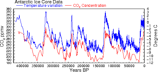Fig. 2 This is the famous graph showing correlation between CO₂ and temperature [31]. The calculations above show that much of this correlation can be explained by the fact that warmer temperatures cause CO₂ to be released or 'outgassed' from the oceans.

The calculations do not rule out other factors. For example, acidification of the oceans by acid rain lowers the solubility of CO₂ and causes outgassing. Ocean currents that circulate deep, CO₂-rich water toward the surface also cause outgassing. The presence of calcium and magnesium ions also affect the carbonate-bicarbonate equilibrium by forming insoluble carbonates. Calculating the amount of outgassing produced by all these factors is tricky.

In the laboratory, if the partial pressure of CO₂ is high enough (>1.26 MPa at 0°C), CO₂ can form a hydrate, which is an unstable clathrate similar to that formed from methane. Clathrates can store prodigious amounts of gas. CO₂ clathrates are not known to occur in the ocean. However, volcanoes release large amounts of carbon dioxide, which can remain trapped by water under pressure and then released unpredictably and catastrophically, as happened in 1986 in Lake Nyos in Cameroon [30].

It should be mentioned that Henry's law does not work well for CO₂ at high pressure, such as might be found on Venus or in a soda bottling plant; in this case, the Krichevsky-Kasarnovsky equation [27] is needed to calculate the solubility. This equation adds an extra term that corrects for the pressure effects. But for ocean surface pressures, Henry's law is adequate. (note added 1/08/2010)

Technically, these calculations should use activity and not concentration for more accurate results. However, for the concentrations involved here, the differences will be small. (note added 2/12/2010)

Figures from the U.S. Department of Energy show that the pre-industrial baseline of carbon dioxide is 288 parts per million by volume (ppmv). The current level of carbon dioxide is 368.4 ppm, or 0.0368% of the atmosphere. For a gas, one part per million by volume means there is one molecule for every million molecules of all other gases. One ppmv gives the same partial pressure for any gas; because of the ideal gas law (pV = nRT), this partial pressure is independent of its molecular weight.

The ocean and biosphere possess a large CO₂ buffering capacity, mainly because of carbon dioxide's large solubility in water. Because of this, it is safe to conclude that the anthropogenic component of atmospheric carbon dioxide concentration will continue to remain roughly proportional to the rate of carbon dioxide emissions for any conceivable rate of human emission. In other words, the carbon dioxide buffers are in dynamic equilibrium with atmospheric carbon dioxide and are not in any danger of being saturated, which would allow all the emitted carbon dioxide to go into the atmosphere. This means:

• The percentage of emitted carbon dioxide that ends up in the atmosphere can be treated as approximately constant. This percentage is about 50% [6] (other sources place it closer to 45%). However, the buffering capacity of the oceans is enormous. The oceans currently contain about 50 times as much CO₂ as the atmosphere [20].
• The effects of carbon dioxide emissions are not cumulative. That is, lowering carbon dioxide would produce an almost instantaneous reduction (on a climatological scale) in any warming effect that it was producing.
• If fossil fuel use increases or decreases, atmospheric carbon dioxide will also increase or decrease proportionately to the percentage of CO₂ that was man-made.

Comment added 1/5/2008:
This last point has been misinterpreted by some commentators. To clarify, this means that if we were to stop emitting carbon dioxide, the CO₂ levels in the atmosphere would rapidly return to pre-industrial levels. Geologists tell us that the residence time of CO₂ in the atmosphere is on the order of five to ten years [23]. In contrast, the IPCC says it is 50-200 years. Whatever the actual number, there is no question that emitting CO₂ will cause it to accumulate over short periods. But other processes, such as sequestration, also work against it, causing the levels to decrease rapidly over time.

This fact is the very basis of the effort among global warming advocates to lower CO₂ emissions. Indeed, if this were not true, there would be no possible benefit to reducing CO₂ emissions, as CO₂ levels would ratchet up indefinitely, whether by natural or artificial means, without limit.

Amplification and Dampening

Of course, climate, like weather, is complex, nonlinear, and perhaps even chaotic. Increased solar irradiation can lower the surface albedo (reflectivity), which could amplify any effect caused by changes in solar flux, making the relation between radiation and temperature greater than linear. A change in albedo can occur through several factors: (1) at the edges of snow/ice cover, where snow and ice cover bare ground or vegetation for only part of the year, there can be increased periods of snow or of bare ground; (2) as snow cover ages, it changes to ice, which has lower reflectivity; and (3) dust and dirt can land on top of the ice, increasing absorption of light.

Increased temperatures also cause increased evaporation of sea water, which can cause warming because of water's greenhouse effect, and also can cause cooling by creating additional clouds, which reflect more radiation into space. On the other hand, increased plant growth, especially in the oceans, would tend to extract carbon dioxide from the atmosphere, making the fraction of emitted carbon dioxide that stays in the atmosphere lower. Thus, higher emissions would probably cause a slightly smaller proportion of carbon dioxide to remain in the atmosphere than is currently the case, tending to make the relation less than linear.

Absorption of Infrared Radiation

The arithmetic of absorption of infrared radiation also works to decrease the linearity. Absorption of light follows an exponential curve (Fig. 3) as the amount of absorbing substance increases. It is generally accepted that the concentration of carbon dioxide in the atmosphere is already high enough to absorb virtually all the infrared radiation in the main carbon dioxide absorption bands over a distance of less than one km. Thus, even if the atmosphere were heavily laden with carbon dioxide, it would still only cause an incremental increase in the amount of infrared absorption over current levels.

Fig.3. Transmitted light is proportional to the logarithm of the concentration. This is the familiar Beer's Law.

This means that a situation like Venus could not happen here. The atmos­phere of Venus is 90 times thicker than Earth's and is 96% carbon dioxide, making the atmospheric carbon dioxide concentration on Venus 300,000 times higher than on Earth. Even so, the high temperatures on Venus are only partially caused by carbon dioxide; a major contributor is the thick bank of clouds containing sulfuric acid [7]. Although these clouds give Venus a high reflectivity in the visible region, the Galileo probe showed that the clouds appear black at infrared wavelengths of 2.3 microns due to strong infrared absorption [8]. Thus, Venus's high temperature might be entirely explainable by direct absorption of incident light, rather than by any greenhouse effect. The infrared absorption lines by carbon dioxide are also broadened by the high pressure on Venus [9], making any comparison with Earth invalid.

Very little of the radiation from the sun at the wavelengths at which carbon dioxide absorbs reaches the surface of the Earth directly (see Fig. 4) [10]. Similarly, very little of the radiation at these wavelengths that originates at the surface makes it all the way to space. Most of the infrared at these wavelengths is produced by black body radiation from objects that have been heated up by absorbing radiation at shorter wavelengths. This means that even if the carbon dioxide levels increase, it will have little effect on the total amount of infrared radiation that is absorbed from the sun. The main effect would be to trap radiation originating at the surface at night at lower levels in the atmosphere than before, where it would be slightly more difficult for the heat to be re-radiated back into space. This is the principle on which most of the global warming predictions are based.

CO₂ is more evenly distributed than water, so if CO₂ caused warming it would have a proportionately greater effect in areas where there is little water vapor (such as deserts and in very cold regions), while in areas with a lot of water, the effect of CO₂ may be insignificant (in terms of its effect on local temperature) compared to the effect of water vapor. This is one of many factors that mitigate against the idea of a “climate catastrophe.” [16]

Beer's law is not perfect. One type of deviation from Beer's law occurs when the medium becomes saturated. When this happens, the molecules are no longer able to absorb light, and the absorbance per unit distance decreases. If the light source is sufficiently intense (a strong laser, for instance), the medium becomes optically transparent [28]. The relative rate of excitation by photons and relaxation by spontaneous emission or molecular collisions determines the actual absorbance.

As one reader pointed out, Beer's law was derived for a single beam of light going through a gas or solution for which the re-emitted radiation does not enter the detector. Therefore, Beer's law will not fit the situation precisely, but there is general agreement that the curve is approximately logarithmic in shape.

The net effect of all these processes is that doubling carbon dioxide would not double the amount of global warming. In fact, the effect of carbon dioxide is roughly logarithmic. Each time carbon dioxide (or some other greenhouse gas) is doubled, the increase in temperature is the same as the previous increase. The reason for this is that, eventually, all the longwave radiation that can be absorbed has already been absorbed. It would be analogous to closing more and more shades over the windows of your house on a sunny day—it soon reaches the point where doubling the number of shades can't make it any darker.

Another way of looking at it is by thinking of adding blankets to your bed on a cold night: if you have no blankets, adding one will have a big effect. If you have a thousand blankets, adding another thousand will have an unmeasurably small effect.

The analogy with a greenhouse would be that the glass in the roof becomes slightly thicker. The effect of warming also depends on the conditions inside the greenhouse. If the greenhouse were full of ice at exactly −0.01°C, making the glass slightly thicker just might be enough to melt all the ice and flood the greenhouse. But if the greenhouse had some regions that were hot and some that were very cold (as the planet Earth does), it would have a very small overall effect.

As an aside, the term “greenhouse effect” is actually a misnomer. In greenhouses, most of the warming that is observed is not caused by carbon dioxide, or by absorption of infrared radiation by the glass as many people think, but by reduction in convection [11].

Fig.4. Absorption of ultraviolet, visible, and infrared radiation by various gases in the atmosphere. Most of the ultraviolet light (below 0.3 microns) is absorbed by ozone (O3) and oxygen (O2). Carbon dioxide has three large absorption bands in the infrared region at about 2.7, 4.3, and 15 microns. Water has several absorption bands in the infrared, and even has some absorption well into the microwave region. There is already sufficient CO₂ in the atmosphere to absorb almost all of the radiation from the sun or from the surface of the earth in the principal CO₂ absorption bands. (Data from ref. [1], page 93; original data are from Howard et al [21] and Goody [22]).

What does 'saturation' mean?

Many people seem to be confused about the “saturation” argument. It's easy to calculate, using the known extinction coefficients [10], that almost all of the radiation in the CO₂ absorption bands is absorbed within only a few meters of the source. These coefficients are derived from measurements in modern, high-resolution spectrometers. But strong absorption is also found even with older, lower-resolution instruments. So what does this mean? Is the global warming theory false? Or should older measurements not be trusted? Here is what it means:

1. The “saturation” argument does not mean that global warming doesn't occur. What saturation tells us is that exponentially higher levels of CO₂ would be needed to produce a linear increase in absorption, and hence temperature. This is basic physics. Beer's law has not been repealed.
   
2. Some people have gotten the idea that water vapor, which is mainly present at lower altitudes, is somehow necessary for the CO₂ to absorb infrared radiation, and that therefore at higher altitudes, CO₂ is not anywhere near saturation. This is not true. The presence or absence of water vapor has no bearing on whether radiation is absorbed by CO₂. That is because, for all practical purposes, the absorption bands of H₂O and CO₂ important for warming are different. (If they weren't, CO₂ absorption would be so insignificant compared to water vapor that it wouldn't be a potential problem, and we wouldn't be having this discussion.)
   
3. CO₂ is very nearly homogeneous throughout the atmosphere, so its concentration (as a percentage of the total) is about the same at all altitudes. Although the pressure is lower at high altitudes, there is also a much greater volume. That is why the ozone layer, which is around 30-90 km in altitude, is still able to absorb almost all of the shortwave UV, even though its concentration is only 8-12 ppm. So the importance of low concentrations of gases should not be underestimated. But water vapor is a red herring: it has essentially no effect on what CO₂ does. Where water vapor becomes important is in the earth's response to CO₂.
   
4. Some people also think that line broadening of the CO₂ absorption lines by pressure, water vapor, or temperature provides an escape from the saturation dilemma. But in line broadening, the absorbance peak is only smeared out; the total amount of energy absorbed is not affected. For the same reason, measurements with lower-resolution spectrometers, which slightly smear out the absorption lines, are still valid.

Saturation does not tell us whether CO₂ can raise the atmospheric temperature, but it gives us a powerful clue about the shape of the curve of temperature vs. concentration.

Calculating the actual temperature increase

So, what is the actual increase? Interestingly enough, that is easy to estimate—and without resorting to complex computer models. In this section we will assume, for the sake of argument, that the CO₂ and temperature readings from the IPCC are correct, and ask: if there is a causal relationship between temperature and CO₂, what is the maximum size the effect could be?

Because a linear increase in temperature requires an exponential increase in carbon dioxide (thanks to the physics of radiation absorption described above), we know that the next two-fold increase in CO₂ will produce exactly the same temperature increase as the previous two-fold increase. Although we haven't had a two-fold increase yet, it is easy to calculate from the observed values what to expect, assuming the correlation represented a cause and effect relationship.

Between 1900 and 2000, atmospheric CO₂ increased from 295 to 365 ppm, while temperatures increased about 0.57° (using the value cited by Al Gore and others). It is simple to calculate the proportionality constant (call it 'k') between the observed increase in CO₂ and the observed temperature increase:

This shows that doubling CO₂ over its current values should increase the earth's temperature by about 1.85°. Doubling it again would raise the temperature another 1.85°. Since these numbers are based on actual measurements, not models, they include the effects of amplification, if we make the reasonable assumption that the same amplification mechanisms that occurred previously will also occur in a world that is two degrees warmer.

If we want to include other greenhouse gases, such as methane, in the calculation, we need to use the “effective” CO₂ concentrations instead. These effective CO₂ numbers are less solid than the CO₂-only numbers, but the best estimates are that effective CO₂ increased from 305 to about 450 ppm during the 20th century[12]. Using these numbers, k becomes 0.6823 and the predicted ΔT becomes 1.02 degrees.

These estimates assume that the correlation between global temperature and carbon dioxide is causal in nature. This remains to be proved. Therefore, the 1.02 and 1.85 degree estimates should also be regarded as upper limits.

Refinements to the estimate

Unfortunately, the above calculations slightly overestimate the degree of warming, because they allow the temperature to rise indefinitely. At very high CO₂ levels, self-absorption would become a limiting factor. A more accurate calculation is shown below.

A reader named Ted Ladewski made an interesting suggestion: use the 255K zero-greenhouse gas data point, where there is zero CO₂, as a data point, and fit the other points to a smooth curve. To maximize the accuracy of the estimate, we will only use global CO₂ and temperature values between 1900 and 2000 [14], about which there is relatively little dispute, and ignore estimates of prehistoric values, which could be more affected by changes in solar flux and other factors. This gives a total of 102 data points. These points are shown in blue in the figure below.

Including the CO₂ = 0 data point severely constrains the shape of the curve (and, interestingly, effectively rules out any sort of hockey stick-shaped curve). It is also clear that some sort of monotonically-increasing curve, and not a straight line, has to be used. The best fit was obtained with a hyperbola. If the 102 data points are fitted to a hyperbola, we obtain 288.92 ±0.27K (±1 SD) for 736 ppm CO₂ (red line).

The present-day value is taken as the average of the global mean temperatures between 1980 and 2000, or 287.17K. If the above estimate is correct, this means that the temperature would increase by 1.76±0.27°C above the present-day value when CO₂ levels double their present levels. This is very close to the 1.85°C calculated above.

Stated differently, doubling CO₂ from its pre-industrial value would increase the temperature about 1.2°C.

Fig. 5.

However, there is a problem with this method. The 255K data point is not just zero CO₂, it is zero water vapor as well. In reality, there would always be some water vapor present, even if there were no CO₂. This means that the actual temperature for zero CO₂ would be higher than 255K, which would change the shape of the curve. For example, if the CO₂=0 value was 271 (halfway between 255 and the current temperature), the prediction changes to 288.55K, or about a 1.39 degree increase for doubling of CO₂. This can be seen in the blue curve (see enlarged graph below). The result is not much different than the 1.76, but the important point is that as the estimates become more realistic, the predicted temperature does not increase, but decreases slightly.


Fig. 6.

Fitting other curves to these data points gives similar results. For example, Ted Ladewski suggested deriving an exponential curve from Beer's Law. Although there are obvious problems involved in applying Beer's Law quantitatively to a transparent medium as complex as the atmosphere (as he discusses in greater detail on his website, http://mysite.du.edu/~etuttle/weather/atmrad.htm#Spec), the equation he recommends is:

where AIo and k are constants, C is the CO₂ concentration, and T is temperature. (This is also discussed in http://www.sjsu.edu/faculty/watkins/GWnonlinear.htm )

Fitting the data to this equation, as shown in the brown curve in the figure above, gives the much lower value of 287.62±0.07 K (±1 SD), or 0.46±0.08 °C increase above the 1980-2000 mean for a doubling of CO₂ from current values.

Although extrapolating beyond the ends of the data, as is done here and as is done with climate models, is hazardous, it's clear that both of these curves are significantly lower than a straight linear estimate. The hyperbola is probably closest to the actual value, because it makes the fewest assumptions about the underlying physical processes. In any case, both estimates should be regarded as upper limits because, as mentioned above, they assume that CO₂ is the root cause of the observed changes in temperature.

How long will it take to double CO₂ levels?

Another issue that people are confused about is the rate of increase of carbon dioxide. Some people think that CO₂ is rising dramatically. This is probably because of graphs like the one below.

Fig. 7.

However, in hard science journals, the graph above would be considered dishonest, because the y-axis starts at 290 instead of zero. This misleads the reader into thinking that CO₂ levels have undergone a huge increase when in fact, CO₂ levels have only increased by 23.7% since 1900. When the data are plotted honestly, with the y axis starting at zero, the true scope of the change becomes clear.

Fig. 8.

According to the US Department of Energy, about 14.8% of the total CO₂ is man-made. The remainder is caused by natural forces, such as volcanoes and forest fires [25].

At the current rate of increase, CO₂ will not double its current level until 2255.

Fig. 9.

Some climatologists, making assumptions about ever-increasing rates of carbon dioxide production, assert that the doubling will occur within a few decades instead of a few centuries. However, they are doing sociology, not climatology. They are assuming that fossil fuel consumption will increase drastically over current levels. This is very unlikely. The only honest way to estimate the change of CO₂ levels is to make predictions based on what is happening now, not what might happen in some hypothetical future society; otherwise, we are merely inflating our predictions by indulging in speculation about future social trends.

Many people have used tricks like these to exaggerate the amount of global warming, and this has made it into a political issue. Most people would have great difficulty feeling an increase of 0.6°C. Any effects of such a small change would be slow and subtle. In general, if you are able to see or feel some change, that means it is almost certainly not caused by CO₂-induced global warming.

Secondary effects

What about secondary effects, such as ice melting, changes in albedo, and so forth? Doesn't this increase the predicted temperature beyond the 1.39 to 1.76 degree estimate?

In short, no. Because these calculations are based on observed measurements, they automatically take into account all of the earth's responses. Whatever way the climate adapted to past CO₂ increases, whether through melting, changes in albedo, or other effects, is already reflected in the measured temperature, and therefore it will also be reflected in the prediction. This is because the prediction is based on an extrapolation of past measurements that were taken after the earth adapted to the CO₂ increase.

In order to get higher temperatures than those predicted above, it would be necessary to assume that a small increase in warming causes a large change in the amplification effect that had never occurred before. In other words, the “rules of the game” would have to drastically and abruptly change in a fundamentally new way—in response to an increase of only one or two degrees. Such changes do not occur in the real world—only in computer models. (If these so-called “tipping points” existed, random, day-to-day, and seasonal variability would have pushed us past them a long time ago.)

This is what makes the “empirical” method superior to all the computer models, as sophisticated as they may be. The empirical model just looks at what's happening and makes a reasonable extrapolation, with very few prior assumptions. The only drawback of the empirical method is that it can only predict an upper limit, because it does make one big assumption: that correlation implies causality. Therefore, although the actual warming cannot be greater than the predicted estimate, it could be considerably less.

Masking

Some climatologists may object to the foregoing analysis, pointing out that the effects of an increase in CO₂ could be masked by sulfate aerosols or other factors. For example, the eruption of Mount Pinatubo in 1991 released large amounts of volcanic aerosols that may have been responsible for a brief global cooling [18]. However, later studies showed that water vapor feedback was necessary to account for this effect [19]. Applied to global warming, the reasoning is that human sulfate emissions might “mask” warming by cooling the atmosphere. In the future, they say, sulfate emissions might decrease while CO₂ remains constant, and the true global warming would be revealed.

The problem here is that trying to account for sulfates drags us into the morass of modeling of social trends. It is much more reasonable to assume that, as industry shifts production to developing countries and people use more coal and high-sulfur oil to replace dwindling supplies, that sulfate emissions will greatly increase. Additionally, sulfates are only one factor. Many other factors, even including such things as cosmic rays, have been shown to have potential effects on climate. Some of these hypothetical effects would cause warming and some would cause cooling. We need to focus on what can be measured directly. The only issue is whether CO₂ is a problem. To add or subtract these myriad hypothetical effects, and claim that the actual amount of warming that is occurring is different from the warming that can be observed, only serves to take climatology that much closer to metaphysics.

One reader pointed out a similar factor that is sometimes mentioned: the heat absorbing capacity of the oceans. Water has 4.13 times the heat capacity of air on a weight basis at 25°C (2.58 times on a molar basis). The oceans contain 273 times as much mass as the atmosphere, and the top few meters alone can store as much heat energy as the entire atmosphere. Thus, much of the extra heat is undoubtedly going into the oceans. But what does this really mean? If the oceans masked all the warming by absorbing the heat, we would have to multiply the time scale by about 1128 before we see the real warming. That means warming that we thought would occur over a 250-year time period would actually take 250×1128 = 282,000 years. By then, humans will almost certainly be getting their energy from some other source besides combustion of hydrocarbons. And then there is the earth's crust, which can absorb additional heat over a scale of billions of years.

Linear Climate Projections

An alternative way of calculating future temperature increases is to consider the fraction of warming that is caused by CO₂. To do this, we cannot just use the fraction of radiation that is absorbed by CO₂, because that does not take feedback processes into account.

As a first step, let us suppose that temperature increases linearly with greenhouse gas concentrations. From the above numbers, it is easy to calculate that a doubling of atmospheric carbon dioxide would produce an additional warming of (0.042 to 0.084) x 33 = 1.38 to 2.77 degrees centigrade. This is the temperature change one would expect that if CO₂ doubles over its current levels.

It is important to realize that the original factor of 0.042 to 0.084 used in these calculations represents the incremental fraction of the total global warming, taken as a holistic phenomenon, initiated by carbon dioxide. This means that the calculation automatically includes the secondary and amplification effects caused by increased water vapor, changes in albedo, and so forth, caused by including the Earth's adaptation to the increment of carbon dioxide.

Fig. 10. Estimated greenhouse gas-induced global warming plotted against greenhouse gas concentrations expressed as a percentage of current-day values. The black curve is a linear extrapolation calculated from the DOE estimates of total current greenhouse gases. The sharp jump at the right is the data point from one computer model that predicts a nine degree increase from doubling current levels of carbon dioxide. Marked, unphysical deviations from linearity resulting in thermal runaway (red curve) are required to fit this data point with the two known points. Such a strong nonlinear effect is difficult to reconcile with our current understanding of climate.

However, our results are based on the assumption that the increase in temperature is linearly proportional to the greenhouse gas levels. This is not true. The relationship is not linear, but logarithmic. If we plot temperature vs. gas concentration (expressed as a percentage of current-day levels), we obtain a convex curve, something like the blue curve in Fig. 10. Thus, the 1.4-2.7 degrees obtained from our linear estimate is an upper bound, and depending on the exact shape of the blue curve, could be a large overestimate of the warming effect.

It goes without saying that the results from this method depend on the accuracy of the 5% estimate (from ref. [3]) and the validity of extrapolating the existing curve by an additional increment. The exact number is very difficult to pin down.

Whether the exact number is 5% or 9%, because our estimate is based on the percentage of warming, not percentage of radiation absorbed, that is attributable to CO₂, feedbacks in the estimate here are automatically taken into account. However, because of the large uncertainty about the actual value, the estimate from Fig. 5 (which derives an estimate from extrapolation of current trends) is probably more accurate.

However, we can also check the plausibility of the IPCC's result by asking the following question: What number would result if we calculated backwards from the IPCC estimates?

Using the same assumption of linearity, if a 9 degree increase resulted from the above-mentioned increase of greenhouse gas levels, the current greenhouse gas level (which is by definition 100%) would be equivalent to a greenhouse gas-induced temperature increase of at least 107°C. This means the for the 9 degree figure to be correct, the current global temperature would have to be at least 255 + 107 − 273 = 89°C, or 192° Fahrenheit! A model that predicts a current-day temperature well above the highest-ever observed temperature is clearly in need of serious tweaking. Even a 5 degree projection predicts current-day temperatures of 41°C (106°F). These results clearly cannot be reconciled with observations.

In order for the 9 degree estimate to make sense from a physical standpoint, we are forced to draw an exponential curve through the graph above (shown in red) through the three points instead of a straight line. However, this curve creates an even worse result: it predicts a thermal runaway. A thermal runaway is a reaction that suddenly switches from a smooth curve and goes wildly out of control. For the the nine-degree climate model to fit the observations, the curve that we must draw predicts that a 10 or 20% increase in greenhouse gases above their current levels would cause an infinite increase in temperature! Of course, some other factor (such as explosion of the Earth in a supernova-type explosion) would undoubtedly kick in to save us before an infinite temperature could be reached. But even so, it can be seen that an above-linear increase in temperature with increasing gas concentration is not only unphysical, but inconsistent with observations.

Although the estimates of global warming made by the IPCC and the predictions of “environmental catastrophe” made by environmental groups have gradually creeping back down as climate models gradually improve, environmentalists still worry that temperatures could increase by as much as 3 to 5 degrees over the next century.

However, even a 5 degree increase in temperature over the next century would constitute a significant departure from the previous rates of increase. It is clear from Fig. 10 that this too would be a marked deviation from the curve. Such strong nonlinear effects, especially when they are in the wrong direction from a physical standpoint, are difficult to reconcile with our current understanding of climate.

Conclusion

Although carbon dioxide is capable of raising the Earth's overall temperature, the IPCC's predictions of catastrophic temperature increases produced by carbon dioxide have been challenged by many scientists. In particular, the importance of water vapor is frequently overlooked by environmental activists and by the media. The above discussion shows that the large temperature increases predicted by many computer models are unphysical and inconsistent with results obtained by basic measurements. Skepticism is warranted when considering computer-generated projections of global warming that cannot even predict existing observations.

References and Notes

[1]. Peixoto, J.P. and Oort, A.H., Physics of Climate Springer, 1992, p. 93 and 118.
[2]. Thomas, G.E. and Stamnes, K. Radiative Transfer in the Atmosphere and Ocean. Cambridge University Press, 1999, p. 441.
[3] Most credible sources place the number at 95%.
95% = Michaels, P.J. and Balling, R.C., The Satanic Gases. Cato Institute, 2000 p.25.
90-95% = http://www.globalwarming.org/node/62
90% = http://www.ncpa.org/press/transcript/globalwm/global2.html Norman J. Macdonald Carbon dioxide is about 5 percent, water vapor 90.
Here is a paper that gives a different figure: http://www.atmo.arizona.edu/students/courselinks/spring04/atmo451b/pdf/RadiationBudget.pdf"
S.M. Freidenreich and V. Ramaswamy, Solar Radiation Absorption by Carbon Dioxide, Overlap with Water, and a Parameterization for General Circulation Models. Journal of Geophysical Research 98(1993):7255-7264
[4]. U.S. Climate Action Report 2000, US Environmental Protection Agency, page 38.
[5]. Houghton, J.T. et al, eds. Climate Change 1995: The Science of Climate Change (IPCC report), 1996, Cambridge University Press. http://www.ipcc.ch/pub/sarsum1.htm
[6]. Peixoto, J.P. and Oort, A.H., Physics of Climate. Springer, 1992, p. 436.
[7]. http://www.aas.org/publications/baas/v33n3/dps2001/354.htm
[8]. http://www2.jpl.nasa.gov/galileo/slides/slide3.html
[9]. Ma, Q., and R.H. Tipping, J. Chem. Phys., 96, 8655-8663, 1992.
[10]. [note added Feb 15, 2007] This can be easily calculated from the absorption of gaseous carbon dioxide. See Phys. Rev. 41, 291 - 303 (1932) P. E. Martin and E. F. Barker "The Infrared Absorption Spectrum of Carbon Dioxide".

Thomas and Stamnes (ref. 2, page 91) that shows 0% transmittance at 22 km and below for the 15 micron CO2 band. This section discusses the "opaque region" and also gives a very clear discussion of line broadening, which is an additional point that many people are unfamiliar with.

Schneider, Kucerovsky, and Brannen (Appl. Opt. 28:5, 1998) give an absorption coefficient at 9.90 ± 1.49 cm-1 atm-1 for low concentrations of CO2 in a 1-atm nitrogen atmosphere at 4.2 microns. This works out to 376 absorbance units per km for 380 ppm CO2, which is about as close to 100% absorption as you can get. Heinz Hug measured a similar value (0.03 absorbance units/10 cm for 357 ppm at 15μm) ( http://www.john-daly.com/artifact.htm).

[11]. Peixoto, J.P. and Oort, A.H., Physics of Climate. Springer, 1992, p. 30.
[12]. The Satanic Gases, p.36.
[13]. Carbon dioxide is written here as CO2 instead of CO₂ because using subscripts messes up the line spacing in most browsers. The Unicode character x2082 (₂), which normally solves this problem, doesn't display properly in some versions of Internet Explorer.
[14]. The temperature data for these calculations were obtained from http://lwf.ncdc.noaa.gov/oa/climate/research/anomalies/anomalies.html
[15]. www.realclimate.org
[16]. One reader pointed out that the Arctic region has dew points above freezing during a significant portion of the year. The average desert atmosphere also has a much higher water content than many people think.
[17]. However, some climatologists have tried to invoke anthropogenic increases in atmospheric water vapor: see Santer et al., "Identification of human-induced changes in atmospheric moisture content" (Proc Natl Acad Sci U S A. 2007 Sep 25;104(39):15248-53). Using a computer model, the authors concluded that human activity is increasing water vapor.
[18]. Radiative Climate Forcing by the Mount Pinatubo Eruption. Minnis P, Harrison EF, Stowe LL, Gibson GG, Denn FM, Doelling DR, Smith WL Jr. Science. 1993 Mar 5;259(5100):1411-1415.
[19]. Global cooling after the eruption of Mount Pinatubo: a test of climate feedback by water vapor. Soden BJ, Wetherald RT, Stenchikov GL, Robock A. Science. 2002 Apr 26;296(5568):727-30.
[20]. http://www.aip.org/history/climate/oceans.htm This is a pro-global warming website.
[21]. Howare, J.N., Burch, D.L., Williams, D (1955). Near-infrared transmission through synthetic atmospheres. Geophys. Res. Papers No. 40, Geophys, Res. Dir., Air Force Cambridge Research Center, 244 pp.
[22]. Goody, R.M. (1964). Atmospheric Radiation: I. Theoretical Basis. Clarendon, Oxford, 436 pp.
[23]. National Academy of Sciences, Climate Research Board (1979). Carbon dioxide and climate: a scientific assessment. National Academy of Sciences, 72pp.; cited in Ref. 1, p. 434.
[24]. See also: Steven Goddard, Divergence Between GISS and UAH since 1980 and
Oceans are cooling according to NASA (non-technical newspaper article).
[25]. Current Greenhouse Gas Concentrations (updated October, 2000) Carbon Dioxide Information Analysis Center, U.S. Department of Energy Oak Ridge, Tennessee
[26]. Fred Goldberg (2008). Rate of Increasing Concentrations of Atmospheric Carbon Dioxide Controlled by Natural Temperature Variations. Energy & Environment, Volume 19, Number 7, pp. 995-1011, December 2008. Available online
[27]. Carroll J.J. and Mather, A.E. (1992) The system carbon dioxide-water and the Krichevsky-Kasarnovsky equation Journal of Solution Chemistry Volume 21, Number 7 / July, 1992, p.607-621
[28]. Ronald G. Driggers, Encyclopedia of Optical Engineering, Vol. 2, page 1475. Marcel Dekker, 2003.
[29]. Gerhard Gerlich, Ralf D. Tscheuschner (2007). Falsification Of The Atmospheric CO2 Greenhouse Effects Within The Frame Of Physics. arXiv:0707.1161v4 [physics.ao-ph]
[30]. http://pagesperso-orange.fr/mhalb/nyos/nyos.htm
[31]. Petit, J.R., J. Jouzel, D. Raynaud, N.I. Barkov, J.-M. Barnola, I. Basile, M. Bender, J. Chappellaz, M. Davis, G. Delayque, M. Delmotte, V.M. Kotlyakov, M. Legrand, V.Y. Lipenkov, C. Lorius, L. Pepin, C. Ritz, E. Saltzman, and M. Stievenard. 1999. Climate and atmospheric history of the past 420,000 years from the Vostok ice core, Antarctica. Nature 399: 429-436.
Jouzel, J., C. Lorius, J.R. Petit, C. Genthon, N.I. Barkov, V.M. Kotlyakov, and V.M. Petrov. 1987. Vostok ice core: a continuous isotope temperature record over the last climatic cycle (160,000 years). Nature 329:403-8.
Jouzel, J., N.I. Barkov, J.M. Barnola, M. Bender, J. Chappellaz, C. Genthon, V.M. Kotlyakov, V. Lipenkov, C. Lorius, J.R. Petit, D. Raynaud, G. Raisbeck, C. Ritz, T. Sowers, M. Stievenard, F. Yiou, and P. Yiou. 1993. Extending the Vostok ice-core record of palaeoclimate to the penultimate glacial period. Nature 364:407-12.
Jouzel, J., C. Waelbroeck, B. Malaize, M. Bender, J.R. Petit, M. Stievenard, N.I. Barkov, J.M. Barnola, T. King, V.M. Kotlyakov, V. Lipenkov, C. Lorius, D. Raynaud, C. Ritz, and T. Sowers. 1996. Climatic interpretation of the recently extended Vostok ice records. Climate Dynamics 12:513-521.

Note This article is updated frequently. See here for information about copying or re-posting this document.
This article is also available in PDF format .
Thanks to many readers for pointing out mistakes and making constructive suggestions.